https://arxiv.org/abs/2010.11929


An Image is Worth 16x16 Words: Transformers for Image Recognition at Scale

While the Transformer architecture has become the de-facto standard for natural language processing tasks, its applications to computer vision remain limited. In vision, attention is either applied in conjunction with convolutional networks, or used to rep

arxiv.org

(Inductive Bias란 학습 시에는 만나보지 않았던 상황에 대하여 정확한 예측을 하기 위해 사용하는 추가적인 가정을 의미합니다.)

ViT_발표자료.pdf
1.81MB


약 1주일 전에 최종 신체검사 후에 합격 후에 최종 합격 통보를 받았다.자세한 내용은 보안으로 걸릴 수 있으니 분위기 위주로 작성할 예정이다.


지원공고 확인

지원 공고 확인은 에브리 타임에서 광고하는 것을 보고 지원하게 되었다.

채용공고
채용 프로세스

지원 가능한 대학 3곳을 1순위, 2순위, 3순위로 나눠서 쓰는 것이 가능했다.(대부분 최종 합격 시 1지망으로 보내는 것 같다)
분야는 원래부터 관심이 있던 그래픽스 및 컴퓨터 비전을 선택했다.


설명회

개인적으로 나는 학과 설명회를 안 들어갔다. 원래 들어가려고 생각을 하였으나, 그날에 까먹고 못 들어가 버렸다.
나중에 최종 합격을 하고 알게 된 사실인데 대략적인 인적성 면접에 대한 일정, 형식 등은 설명회에서 이야기해 주었다고 한다. 나는 이를 모르고 인적성 3일 전, 면접 1~2일 전에 급하게 준비한 것 같다. 나 같은 실수는 하지 않았으면 한다.


지원서 작성

지원서 항목은 무난 무난한 느낌이었다.(지원 동기, 지원 직무 협업경험, 지원 직무 대표적인 연구 및 프로젝트, 보유한 skill)  대체적으로 500자 제한이라, 나를 어필할 수 있는 내용을 최대한 압축하는 것이 좋은 것 같다. 지원 항목을 보면 느끼는 점이 AI와 관련된 경험이 없거나 비전공자인 경우에는 쓰기 어려운 것 같다는 느낌이 들었다. 직무관련된 경험을 쓰는 항목이 3개나 되고, 나는 각각의 항목마다 총 3개의 프로젝트를 정리해서 작성했다.
개인적으로 서류에서 합/불을 가릴 것 같다는 느낌은 들지 않았다. 실제로 대부분의 회사에서도 코딩 테스트와 인적성은 다 보게 해주는 느낌이기 때문이다. 


대략적으로 서류 합격 소식은 10일 정도 걸린 것 같다. 사실 학과 설명회를 들어가서 미리 일정을 알았다면 인적성과 코딩 테스트를 준비하겠지만, 나는 서류 합격 메일을 보고 준비해서 3일 정도밖에 시간이 없었다.


인적성/ 코딩 테스트

SD에듀

인적성은 SD 적성검사연구소에서 나온 것을 알라딘 E북으로 구매하였다. 나의 실수로 3일밖에 시간이 없어 최신 기출 유형을 하루 만에 다 풀고, 하루에 한 개씩 모의고사를 풀었다. 그리고 최대한 눈으로 푸는 연습을 했다. 온라인 인적성이니 필기구를 못쓰는 문제가 있기 때문이다.
개인적으로 나는 인적성을 정말 못 풀었다. 실제 시험에서 반타작을 한 것 같다. 그래서 당연히 떨어질 거라 생각했는데, 붙여주는 거 보니 KT도 절대평가 느낌으로 엄청 낮은 점수가 아니면 다 PASS를 주는 것 같다.


코딩 테스트는 프로그래머스 플랫폼을 이용했다. 기존에 나는 삼성전자 문제도 많이 풀었고, 백준에서 골드 1 정도 티어를 가지고 있어서 프로그래머스 플랫폼에 적응하는 훈련만을 했다. 근데 문제가 너무너무 쉽게 나와서(실버 5~3 정도 느낌) 3문제를 해결하는 데 약 20분 정도 걸린 것 같다. 남은 1시간 40분 동안에 검토만 했다.
기존에 연습할 때처럼 문제만 빠르게 풀고 코드를 이쁘게 정리 안 했는데, 시간 남으면 정리하는 것이 좋은 것 같다.

대충 합격 소식은 시험을 보고 1주일도 안 돼서 나왔다.


실무면접

실무면접은 현직에서 일하시는 분들과 진행하는 면접이다.
다대일로 온라인으로 진행했고, 줌으로 하다 보니 시선처리가 엄청 어려웠다.(시선처리가 가장 중요한 듯)
그리고 내가 바보같이 설명회에 안 들어가고, 인적성이 망해서 당연히 떨어질 줄 알고 준비를 안 했다.
그래서 면접 준비를 하루밖에 못했다.(정확히 8시간 정도, 정장도 없었다. ^^)
면접 내용은 보안이므로 자세히 말을 하지는 못하지만, 자기소개서에 작성한 내용 위주로 진행한 프로젝트에 대해서 질문하셨다.
분위기는 엄청 편안했고, 어려운 질문도 많이 하지 않으셨다.
나는 발음도 좋지 않고, 말도 못 하는 편이라 면접을 걱정했지만 다행히 그런 요소들보다 나의 실무능력 위주로 평가하는 느낌이 강했다.

실무면접도 1주일도 안되서 결과가 나왔다.

임원면접

임원면접은 실무면접보다 불편한 분위기? 였다.

다대일로 이또한 온라인으로 진행했고, 줌으로 하다 보니 시선처리가 어려운것을 당연했다.

그리고 실무는 테이블 배치도 엄청 편하게 되어있었지만, 임원면접은 말그대로 드라마에서 보던 대기업 회의장느낌..이였다. (아무래도 임원분들이다보니 그런것 같다.)

그래도 임원분들이 굉장히 친절하셨다. 긴장을 풀어줄려는 노력이 엄청 보였다..(감사하다)

면접 내용은 자소서 내용이 진짜인지 판단하는 느낌이 강했고, 다른 임원면접처럼 나의 성향을 파악하려는 노력을 많이 하셨다. 중간에 번아웃이 있다고 말실수를 했지만, 다행히 임기응변으로 잘 해결한 것도 있다.

그리고 인성질문이 강한 느낌이였다.
꼬리 질문이 상당히 많았고, 하나하나 캐치해서 질문하는 것이 조금 날카로웠지만 원만하게 잘 해결한 것 같다.
임원면접도 1주일도 안 돼서 결과가 나왔다.
결과가 나오면서 학교를 배치해 주고, 학업계획서를 작성해야 한다. 나는 1지망으로 작성한 한양대학교로 배정되었다.

대학원면접

사실 대학원 면접까지 오면 무조건 붙는다는 주변의 반응이 있어서 준비를 하루밖에 안 했다.
실제로 대학원 면접에 가서 느낀 점은 '무조건 붙는다'였다.
한양대학교 전체 면접날이었고, 대기할 때 KT와 LG 계약학과 인원들과 같이 봤다.
다대1면접으로 교수님들이 많이 바쁜 느낌이 강했다.
들어가서 자기소개 후에 성적 증명서만 보고 이 과목이 A+인데 기억나는 것이 있냐고 물어보셨다.
그렇게 질문 하나하나 하고 끝이었다. 대략 5분 정도?
아무래도 앞에서 힘들게 면접을 봐서 배려를 해준 느낌 같기도 했다.

이렇게 프로세스를 진행하고, 대학원 면접 합격을 받았다.
채용검진은 .. 그냥 떨어지면 병원에 가서 입원해야 하는 느낌이 강할 정도로 단조로웠다.
최종 합격하고 나서 느낀 것이지만, 솔직하게 대답하고 나의 역량을 어필하는 것이 중요한 것 같다.
그리고 나처럼 바보같이 채용설명회를 무시하지 말고 정보를 확보하는 것이 좋은 것 같다.


앞으로 2년간 열심히 노력해야겠다. ㅇㅅㅇ..

https://www.acmicpc.net/problem/23291


23291번: 어항 정리

마법사 상어는 그동안 배운 마법을 이용해 어항을 정리하려고 한다. 어항은 정육면체 모양이고, 한 변의 길이는 모두 1이다. 상어가 가지고 있는 어항은 N개이고, 가장 처음에 어항은 일렬로 바

www.acmicpc.net

내가 볼려고 쓰는글 가독성 0

 </p

1
2
3
4
5
6
7
8
9
10
11
12
13
14
15
16
17
18
19
20
21
22
23
24
25
26
27
28
29
30
31
32
33
34
35
36
37
38
39
40
41
42
43
44
45
46
47
48
49
50
51
52
53
54
55
56
57
58
59
60
61
62
63
64
65
66
67
68
69
70
71
72
73
74
75
76
77
78
79
80
81
82
83
84
85
86
87
88
89
90
91
92
93
94
95
96
97
98
99
100
101
102
103
104
105
106
import sys
from collections import deque
N, K = map(int, input().split())
fish_input = list(map(int, input().split()))
fishbowl = deque([deque([fish_input[i]]) for i in range(N)])
 
def push_least_fish():
    min_value = min(fishbowl)[0]
    for index in range(N):
        if min_value == fishbowl[index][0]:
            fishbowl[index][0+= 1
 
def left_fishbowl_push():
    fishbowl[1].extend(fishbowl[0])
    fishbowl[0].pop()
 
def fly_upper2():
    while True:
        left_pop_count = 0
        fly_count = 0
        stack_len = 0
        for i in range(len(fishbowl)):
            if len(fishbowl[i]) == 0:
                left_pop_count += 1
            elif len(fishbowl[i]) >= 2:
                stack_len = max(len(fishbowl[i]),stack_len)
                fly_count += 1
        fly = deque()
        for _ in range(left_pop_count):
            fishbowl.popleft()
        if stack_len > len(fishbowl) - fly_count:
            break
        for _ in range(fly_count):
            fly.append(fishbowl.popleft())
        while len(fly) != 0:
            pop_value = fly.pop()
            for _, value in enumerate(pop_value):
                fishbowl[_].append(value)
 
def fish_split():
    dx = [0,1,0,-1]
    dy = [1,0,-1,0]
    new_fish_bowl = deque()
    make_map = [[0 for i in range(len(fishbowl[0]))] for j in range(len(fishbowl))]
 
    for i in range(len(fishbowl)):
        for j in range(len(fishbowl[i])):
            make_map[i][j] = fishbowl[i][j]
    value_info = []
    # print(fishbowl)
    for i in range(len(fishbowl)):
        for j in range(len(fishbowl[i])):
            total_count = 0
            for dx_,dy_ in zip(dx,dy):
                new_x = i + dx_
                new_y = j + dy_
                if new_x >= 0 and new_y >= 0 and new_x < len(fishbowl) and new_y < len(fishbowl[0]) and make_map[new_x][new_y] != 0:
                    minus = abs(make_map[new_x][new_y] - make_map[i][j])
                    # print(i,j,new_x,new_y)
                    # print(make_map[i][j],minus,minus // 5)
                    if make_map[new_x][new_y] > make_map[i][j]:
                        total_count += minus // 5
                    else:
                        total_count -= minus // 5
            value_info.append(total_count)
    index = 0
    for i in range(len(fishbowl)):
        for j in range(len(fishbowl[i])):
            fishbowl[i][j] += value_info[index]
            index += 1
 
def make_line():
    global fishbowl
    new_fish_bowl = deque()
    for index in range(len(fishbowl)):
        for _ in fishbowl[index]:
            dq = deque()
            dq.append(_)
            new_fish_bowl.append(dq)
    fishbowl = new_fish_bowl
 
def repeat_upper():
    number = N
    number = number // 2
    for i in range(number):
        fishbowl[-1 - i].append(fishbowl.popleft()[0])
    number = number // 2
    for i in range(number):
        value = fishbowl.popleft()
        fishbowl[-1 - i].append(value[1])
        fishbowl[-1 - i].append(value[0])
 
answer = 0
while True:
    answer += 1
    push_least_fish()
    left_fishbowl_push()
    fly_upper2()
    fish_split()
    make_line()
    repeat_upper()
    fish_split()
    make_line()
    if max(fishbowl)[0- min(fishbowl)[0<= K:
        print(answer)
        break
cs

https://www.acmicpc.net/problem/23290


23290번: 마법사 상어와 복제

첫째 줄에 물고기의 수 M, 상어가 마법을 연습한 횟수 S가 주어진다. 둘째 줄부터 M개의 줄에는 물고기의 정보 fx, fy, d가 주어진다. (fx, fy)는 물고기의 위치를 의미하고, d는 방향을 의미한다. 방향

www.acmicpc.net

개인 기록용


1
2
3
4
5
6
7
8
9
10
11
12
13
14
15
16
17
18
19
20
21
22
23
24
25
26
27
28
29
30
31
32
33
34
35
36
37
38
39
40
41
42
43
44
45
46
47
48
49
50
51
52
53
54
55
56
57
58
59
60
61
62
63
64
65
66
67
68
69
70
71
72
73
74
75
76
77
78
79
80
81
82
83
84
85
86
87
88
89
90
91
92
93
94
95
96
97
98
99
100
101
102
103
104
105
106
107
108
109
110
111
112
113
114
115
116
117
import sys
from collections import deque
import copy
# input 처리
sys.stdin = open("input.txt","rt")
# 물고기 수 M, 상어 마법 연습 S
M, S = map(int,input().split())
# 초기 입력 fish_pos
fish_pos = deque()
for _ in range(M):
    fish_pos.append(list(map(int,input().split())))
# 상어 위치
sx, sy = map(int,input().split())
 
# dx, dy
dx = [00-1,-1,-10111]
dy = [0,-1-101110,-1]
fish_map = [[[] for i in range(5)]for j in range(5)]
smell_map = [[0 for i in range(5)]for j in range(5)]
def check_range(new_x, new_y):
    if new_x >= 1 and new_x <= 4 and new_y >= 1 and new_y <= 4:
        return True
    else:
        return False
 
def rotete_direction(x,y,dire):
    first = dire
    while check_range(x+dx[dire], y + dy[dire]) == False or (sx == x + dx[dire] and sy == y + dy[dire]) or smell_map[x+dx[dire]][y+dy[dire]] < 0:
        dire -= 1
        if dire == 0:
            dire = 8
        if first == dire:
            return x, y , first
    x = x + dx[dire]
    y = y + dy[dire]
    return x, y, dire
 
def print_map(map_):
    for i in map_[1:5]:
        print(i[1:5])
    print("_"*20)
 
def move_fish():
    global  fish_map
    # print(fish_pos)
    fish_original = fish_map
    fish_map_after = [[[] for i in range(5)] for j in range(5)]
    for i in range(1,5):
        for j in range(1,5):
            arr = fish_map[i][j]
            for value in arr:
                x,y,dire = value[0] , value[1],value[2]
                x,y,dire = rotete_direction(x,y,dire)
                fish_map_after[x][y].append([x,y,dire])
    fish_map = fish_map_after
    return fish_original, fish_map
 
def move_shark(fish_map,fish_original):
    # 상1, 좌2, 하3, 우4
    global fish_pos
    global sx,sy
    shark_move = deque()
    dx_shark = [0,-1,0,1,0]
    dy_shark = [0,0,-1,0,1]
    x, y = [0*3, [0* 3
    for i in range(1,5):
        x[0= sx + dx_shark[i]
        y[0= sy + dy_shark[i]
        if check_range(x[0],y[0]) == False:
            continue
        for j in range(1,5):
            x[1= x[0+ dx_shark[j]
            y[1= y[0+ dy_shark[j]
            if check_range(x[1], y[1]) == False:
                continue
            for k in range(1,5):
                x[2= x[1+ dx_shark[k]
                y[2= y[1+ dy_shark[k]
                if check_range(x[2], y[2]) == False:
                    continue
                count = 0
                for move in set(zip(x,y)):
                    count = count + len(fish_map[move[0]][move[1]])
                x_ = x.copy()
                y_ = y.copy()
                if len(shark_move) == 0:
                    shark_move.append([x_,y_,count])
                elif shark_move[0][2< count:
                    shark_move.appendleft([x_,y_,count])
    sx = shark_move[0][0][2]
    sy = shark_move[0][1][2]
 
    for i in range(1,5):
        for j in range(1,5):
            if smell_map[i][j] < 0:
                smell_map[i][j] += 1
 
    for move in zip(shark_move[0][0],shark_move[0][1]):
        if len(fish_map[move[0]][move[1]]) > 0:
            smell_map[move[0]][move[1]] = -2
            fish_map[move[0]][move[1]].clear()
 
    for i in range(1,5):
        for j in range(1,5):
            fish_map[i][j].extend(fish_original[i][j])
 
 
for i in fish_pos:
    fish_map[i[0]][i[1]].append(i)
for i in range(S):
    fish_original, fish_map = move_fish()
    move_shark(fish_map,fish_original)
answer = 0
for i in range(1,5):
    for j in range(1,5):
       answer += len(fish_map[i][j])
print(answer)
cs

https://www.acmicpc.net/problem/23288


23288번: 주사위 굴리기 2

크기가 N×M인 지도가 존재한다. 지도의 오른쪽은 동쪽, 위쪽은 북쪽이다. 지도의 좌표는 (r, c)로 나타내며, r는 북쪽으로부터 떨어진 칸의 개수, c는 서쪽으로부터 떨어진 칸의 개수이다. 가장 왼

www.acmicpc.net

오랜만에 다시 공부하면서 Python으로 문제를 푸는데 흠.. 아직 코드 정리를 잘 못하겠네요.


1
2
3
4
5
6
7
8
9
10
11
12
13
14
15
16
17
18
19
20
21
22
23
24
25
26
27
28
29
30
31
32
33
34
35
36
37
38
39
40
41
42
43
44
45
46
47
48
49
50
51
52
53
54
55
56
57
58
59
60
61
62
63
64
65
66
67
68
69
70
71
72
73
74
75
76
77
78
79
80
81
82
83
84
import sys
from collections import deque
 
N, M, K = map(int,input().split())
graph = []
# 1번 윗면 2번 북족 3번 동쪽 4번 서쪽 5번 남쪽 6번 아래면
dice = [0,1,2,3,4,5,6]
# 0  1  2  3
# 북 동 남 서
direction = 1
# 전 후
change_dice = [
    [[6,5],[5,1],[1,2],[2,6]],
    [[4,1],[1,3],[6,4],[3,6]],
    [[2,1],[1,5],[5,6],[6,2]],
    [[1,4],[3,1],[4,6],[6,3]],
]
dx = [-1,0,1,0]
dy = [0,1,0,-1]
pos = [0,0]
score = 0
map_score = [[0 for i in range(M)] for j in range(N)]
#print(map_score)
def cal_score():
    for i in range(N):
        for j in range(M):
            dq_stack = deque()
            if map_score[i][j] == 0:
                value = graph[i][j]
                dq_set = set()
                dq_set.add(str(i)+" "+str(j))
                dq_stack.append([i,j])
                while len(dq_stack) != 0:
                    dq_pop = dq_stack.popleft()
                    x, y = dq_pop[0], dq_pop[1]
                    for dx_,dy_ in zip(dx,dy):
                        new_x = x + dx_
                        new_y = y + dy_
                        if new_x >= 0 and new_x < N and new_y >= 0 and new_y < M:
                            if graph[new_x][new_y] == value and map_score[new_x][new_y] == 0:
                                map_score[new_x][new_y] = 1
                                dq_set.add(str(new_x) + " " + str(new_y))
                                dq_stack.append([new_x,new_y])
 
                value = len(dq_set) * value
                for i_ in dq_set:
                    split_ = i_.split(" ")
                    map_score[int(split_[0])][int(split_[1])] = value


for _ in range(N):
    graph.append(list(map(int,input().split())))
 
cal_score()
answer = 0
for index,i in enumerate(range(K)):
    new_x = dx[direction] + pos[0]
    new_y = dy[direction] + pos[1]
    if new_x >= 0 and new_x < N and new_y >= 0 and new_y < M:
        pass
    else:
        direction = (direction + 2) % 4
        new_x = dx[direction] + pos[0]
        new_y = dy[direction] + pos[1]
    pos[0= new_x
    pos[1= new_y
 
    # 주사위 굴리기
    dict_prev = dice.copy()
    for i in change_dice[direction]:
        dice[i[1]] = dict_prev[i[0]]
 
    # A > B
    if dice[6> graph[pos[0]][pos[1]]:
        direction = (direction + 1) % 4
    elif dice[6< graph[pos[0]][pos[1]]:
        direction = direction - 1
        if direction == -1:
            direction = 3
    answer += map_score[pos[0]][pos[1]]
    #print(pos[0]+1,pos[1]+1,"방향",direction,"아래",dice[6])
print(answer)
cs

https://arxiv.org/abs/1706.03762


Attention Is All You Need

The dominant sequence transduction models are based on complex recurrent or convolutional neural networks in an encoder-decoder configuration. The best performing models also connect the encoder and decoder through an attention mechanism. We propose a new

arxiv.org

Abstract

기존의 Dominant Sequence Transduction Model들은 인코더 디코더를 포함하는 복잡한 Recurrent 또는 CNN 기반
가장 성능이 좋은 모델 또한 Attention 메커니즘을 통해 인코더와 디코더를 연결
저자들은 Recurrence와 Convolution을 완전히 배제한 새로운 Network인 Transformer를 제안
두 개의 Translation Task에서 모델이 우수하고 병렬화되어 훈련시간이 훨씬 적게 소요된다는 것을 보여줌
영어-독일어 번역 작업에서 최고 성능은 물론이고, 영어-프랑스어 번역에서도 8개의 GPU를 이용하여 3.5일간 학습 후 Sota에 달성(기존보다 작은 Training Cost)

1. Introdutction

RNN, LSTM, GRU Network는 Sequence Modeling, Machine Translation 등 분야에서 많이 이용

Recurrent Language Model과 Encoder-Decoder의 Boundary를 넓히기 위해 노력

Recurrent Model을 일반적으로 입력 및 출력 시퀀스에 따라 계산을 진행

단계 별로 계산을 진행하므로 이전 Hidden State Ht-1과 t 순서의 입력이 있어야 함

이런 방식은 순차적 특성으로 인해서 Training 시에 병렬처리에 한계가 존재하고, 메모리 제약으로 인해 더 긴 Sequence Length에서 중요해짐

최근 연구에서는 Factorization Trick,  Conditional Computation을 통해 계산 효율을 높이고, 모델 성능을 높임

하지만 Sequential Computation은 근본적인 제약이 있어 한계가 있음


Attention Mechanisms은 Sequence Modeling 및 Transduction Model의 다양한 부분에서 필수적인 부분이 되어고, Input Output Sequence Distance에 상관없이 Dependencies를 모델링 할 수 있음

몇 가지 특별한 경우를 제외하고 Attention은 Recurrent Network와 같이 사용됨


논문의 저자들은 Recurrence를 피하는 대신 Attention에 전적으로 의존하여 입력과 출력 사이에  Global Dependencies를 도출하는 모델인 Transformer를 제안

모델 병렬화에 큰 효과가 있어 P100 GPU를 이용하여 번역 품질을 개선

2. Background

Sequential Compuation을 줄이기 위해 ByteNet, ConvS2S는 Convolution Neural Network를 기본으로 이용하여 모든 입력과 출력 위치에 대해 hidden representation을 병렬화 (RNN을 CNN으로 표현한 연구)

CNN의 경우 n개의 단어를 문맥으로 파악하려면 드는 시간은 O(n/k)이다. RNN의 경우를 생각해보면 linear하기 때문에 시간은 O(n)

이런 모델들은 Input, Output 위치의 신호를 연관시키는데 필요한 작업수가 많이 늘어나 서로간의 Dependencies를 학습하는게 어려움

Transformer는 이러한 작업의 수를 Constant로 줄여주는 Multi Head Attention을 이용


Self-Attention은 Sequence의 Representation을 계산하기 위해서 Single Sequence내에서 다른 위치와 연관된 Attention

Self-Attention은 다양한 Task에서 성공적으로 이용


End-To-End Memory network는 Sequence-Aligned Recurrence 대신에 Recurrent Attenton Mechanism을 기반으로 하고, QA 및 모델링에서 우수한 성능을 발휘 (Recurrent방식이 Sequence방식보다 좋은성능을 보임)


Transformer는 Self-attention에만 의존한 최초의 Transduction Model

3. Model Architecture

가장 Competitive Neural Sequence Transduction Model은 Encoder-Decoder 형태

Encoder의 경우 Input으로 (x1, ..., xn)을 받아 representations z = (z1, ..., zn), 정보가 담겨있는 z를 생성

Decoder의 경우 z를 입력 받아  (y1, ..., ym)를 생성

각 Step마다 Model을 Auto-regressive하고 동작한다. 즉 Decoder의 출력이 다시 입력으로 들어감


Transformer는 figure1의 왼쪽 및 오른쪽 절반은 각각 Encoder와 Decoder가 쌓여있는 모양

self-attention과 point-wise fully connected layer를 이용하여 전체적인 아키텍처가 완성

3.1 Encoder and Decoder Stacks

Encoder

Encoder는 6개의 같은 Layer가 쌓여있는 모양

각 Layer는 2개의 Sub-Layer를 가짐(Multi-Head Self-Attention, Position-wise fc layer)

각각의 Sub-layer에 Residual-Connection을 추가

그 뒤에 Layer Normalization을 진행 그러므로 각각의 Sub-Layer는 LayerNorm(x + Sublayer(x))

Residual-Connection으로 인해 Input Output의 차원은 dmodel=512로 유지

Decoder

Decoder또한 6개의 같은 Layer가 쌓여있는 모양

각 Layer는 Encoder Layer와 유사하나 Masked-Multi Head Attention이 추가됨

Residual Connection을 추가하고, Layer Normalization을 진행

Masked-Multi Head Attention을 통해 i위치에 대한 Prediction이 i보다 앞에있는, 즉 이전의 출력에 대해 Attention을 구할 수 있음

3.2 Attention

Attention 함수는 Query, key, value, output들이 모두 Vector일 때 ,Query와 key-Value 쌍의 집합을 매핑하는 것으로 설명이 가능
Output은 Value Weight Sum로 게산되며, 여기서 각 Value 값에 할당된 Weight들은 key와 Query의 Compatibility function 에 의해 계산

3.2.1 Scaled Dot-Product Attention

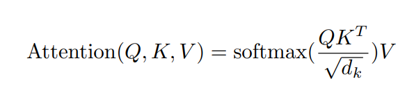
'Scaled Dot-Product Attention'은 위와 같다

input으로 들어오는 Query와 Key의 dimension은 dk이고, Value의 Dimension은 dv

Attention이 궁금한 단어의 Query와 모든 단어의 Key와 Dot-Product를 취하고 루트dk로 나눠준 뒤에 Softmax를 통해 Value에 곱해지는 Weight를 생성, 그 뒤에 Weighted Sum으로 해당 단어와 모든 단어의 Attention을 생성


계산법에는 Additive Attention과 Dot-Product Attention이 존재

Additive Attention의 경우 Single Layer를 통해 Feed Forward로 compatibility function을 계산,

Dot-Product는 dk를 나눠주는것을 제외하면 동일

일반적으로 dk가 작으면 비슷한 성능을 보여주지만, dk가 커질 경우에 softmax에 의해 gradient가 작아지는 문제가 존재하므로 Additive가 좋지만, 해당 논문에서는 dk를 이용해 Scaling ( 기본적으로 Dot-Product는 연산이 매우 가벼움)

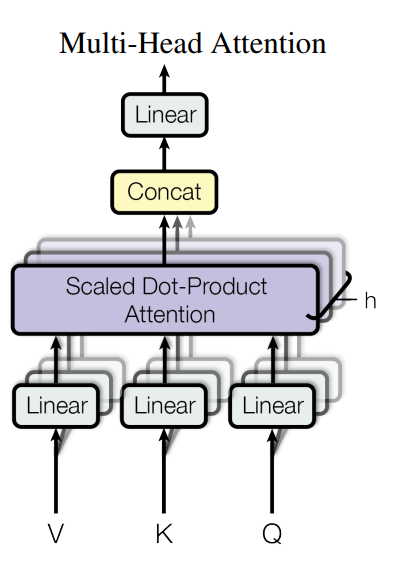
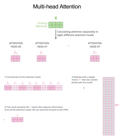
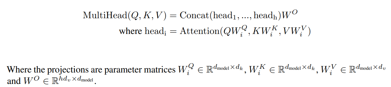
3.2.2 Multi-Head Attention

d-model dimension인 Query, Key, Value로 single attention을 취하는 것보다 h개의 다른 Linear Projection을 취하는 것이 효과적
Multi Head를 통해 모델은 서로 다른 위치에서 서로 다른 Subspace의 Attention을 취함

만약 h = 8 인 경우 dk = dv = dmodel / h = 64로 하여 Single Head Attention과 동일한 연산량을 유지

3.2.3 Applications of Attention in our Model

Transformer는 3가지의 다른 방식으로 Multi-Head Attention을 사용


'Encoder - Decoder Attention' 에서 Query는 이전 Decoder Layer의 출력, Key와 Value는  Encoder의 Output
이를 통해서 Decoder는 Input Sequence의 모든 Position에 대해 Attend가능

Sequence To Sequence Model에서 일반적인 Encoder-Decoder Attention을 모방


Encoder에는 Self-Attention Layer가 포함됨

Self-Attention Layer의 Query, Key, Value는 같은 장소에서 옴

이 경우 Encoder의 이전 Layer의 Output

Encoder의 각 Position은 Encoder의 이전 Layer의 모든 Position에 관여 가능


비슷하게 Decoder또한 Self-Attention Layer를 가짐

Decoder의 Self-Attention 또한 Decoder의 모든 Position에 Attention이 가능

이때 Auto-Regressive한 특성으로 인해 Decoder는 아직 예측하지 못한부분을 Attention하지 못하기 때문에 Masked Self-Attention 진행

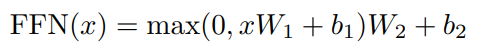
3.3 Position-wise Feed-Forward Networks

Attention Sub-Layer이외에도 Encoder와 Decoder의 각 Layer는 Fully Connected Feed Forward Network가 포함

이 Network는 Activation Function으로 ReLU를 이용하며 W1, W2를 이용해 Linear Transformation을 진행

Input 및 Output Dimension은 dmodel = 512 이고, 내부 Dimension은 dff = 2048

3.4 Embeddings and Softmax

Embedding 같은 경우 다른 Sequence Transduction Model과 비슷하게진행

Input Token과 Output Token을 차원을 dmodel로 변환하기 위해 Training된 Embedding을 이용

그리고 일반적으로 Training된 Linear -Transfomation과 Softmax를 이용하여 구한 Decoder의 출력을 Token 확률로 변환

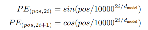
3.5 Positional Encoding

Transformer는 Recurrence와 Convolution도 이용하지 않음, Model이 Sequence를 사용하기 이해 Token의 상대적 또는 절대적 위치에 대한 정보가 필요

이를 위해 Encoder-Decoder Stack 하단 Input Embedding에 Positional Encoding을 추가

Positional Encoding과 Embedding은 같은 차원인 dmodel을 가짐(합치기 가능)

해당 작업에 서로 다른 freq를 가지 sin과 cos을 이용


Pos : Position

i: Token Vector의 차원

Transformer는 Sine을 이용하는데, Model이 더 긴 Sequence 길이를 추론 가능

4. Why Self-Attention

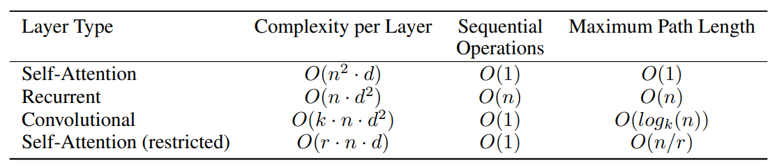
n is the sequence length, d is the representation dimension, k is the kernel size of convolutions and r the size of the neighborhood in restricted self-attention.

해당 Section 에서는 Self-Attention과 Convolution, Recurrent Layer와 비교

3가지를 고려하는데 Computational Complexity Per Layer, Computational Can Parallelized, Long-Range Dependencies 길이


3번째 같은 경우에는 Long-Range Dependencies 사이의 Path 길이
Long-Range Dependency 속성을 하는 것은 Sequence Transduction Task의 핵심

이런 Dependencies를 학습하는 능력에 가장 큰 영향을 미치는 것은 forward, backward path의 길이

input 및 output Sequence의 위치가 서로 가까울수록 Dependencies를 학습하기 쉬움

그러므로 Input과 Output Position을 비교


Table1을 보면 Self-Attention Layer는 모든 Position을 Constant Number로 연결함

하지만 Recurrent Layer 같은 경우 O(n)이 소요

Computational Complexity 관점에서 n이 d보다 작을 경우에  Self Attention 은 Recurrent보다 낮음, 일반적으로 n<d해당

만약 매우 긴 Sequence를 가진 작업에 대해서 성능을 향상시키기 위해 각 input Sequece의 neighborhood size를 r로 제한

이는 maximum path의 길이를 O(n/r)로 증가시킴, 저자들의 Future Work


k < n인 Single Conv Layer는 input과 output의 모든 Pair를 연결 x

Contiguous Kernel의 경우 O(n/k)의 Convolution Stack이 필요

Dilated Convolution의 경우 O(logk(n))이 필요, 계산랑 증가

Convolution Layer는 일반적으로 Recurrent Layer보다 k배 비쌈

근데 Seperable Convolution을 이용하면  

추가적으로 문장의 구조적, 의미적 구조를 잘 연관시킨다

또한 Model이 해석이 가능하고, Attention Map을 시각화하여 왜 이런 결과가 나오는지 해석 가능

주관적인리뷰 이므로 틀린내용이 무조건 존재

https://arxiv.org/abs/1909.13719


RandAugment: Practical automated data augmentation with a reduced search space

Recent work has shown that data augmentation has the potential to significantly improve the generalization of deep learning models. Recently, automated augmentation strategies have led to state-of-the-art results in image classification and object detectio

arxiv.org

RandAugment Paper Review

논문 링크 : https://arxiv.org/abs/1909.13719

Abstract, Introduction

data augmentation은 model의 **generalization(일반화)**을 크게 개선한다. 특히 image classification(분류), object detection(객체탐지) 등 다양한 분야에서 모델 성능 개선에 큰 도움이 된다는 것이 밝혀졌다.

하지만 이러한 Data augmentation은 어려움이 존재한다.

  1. data augmentation을 적용할려는 domain마다 가지고 있는 데이터셋의 특성이 다름.
  2. 그러므로 domain에 **prior knowledge(사전지식)**을 알고 augmentation policy(증강정책) 선택.
  3. 하지만 이러한 prior knowledge를 찾는 것은 어렵고 별도의 Search space가 필요.
  4. 그리고 만약 prior knowledge를 찾더라도 다른 domain으로 확대하는 것은 매우 어려움.

이러한 문제를 해결하기 위해 최근 data augmentation policy를 딥러닝을 통해 찾기 시작하였다.

  1. NAS에서 최적의 Network 아키텍처를 찾는 것 처럼 data augmentation에서도 최적의 policy를 찾을려고 노력 하는 것.
  2. train된 data augmentation policy로 ML model을 학습하는 것은 정확도를 올려주는 경향이 존재.
  3. 하지만 data augmentation policy와 ML model 각각 training 하는 것은 계산량이 많음.
  4. 특히 두개의 분리된 최적화 절차를 수행하는 것은 어려움.

최근에는 PBA, Fast autoaugment에서 효율적인 방식을 제시 하였지만 여전히 문제가 존재한다.

  1. 기존에 존재하던 문제와 마찬가지로 여전히 분리된 최적화 절차가 필요함.
  2. 그리고 작은 데이터셋 학습한 data augmentation policy가 큰 경우에도 적용된다고 가정.
    • 하지만 작은 데이터셋에서 학습한 것을 큰 데이터셋에 그대로 적용하는 것은 문제가 존재.
    • 문제가 발생한 다는 것은 본 논문에서 실험을 통해 보여줌.
    • augmentation을 적용하는 정도는 모델, 데이터셋 사이즈에 의존한다는 것을 확인 가능.

그러므로 본 논문에서는 위에 결과물들을 참고하여 RandAugment를 고안하였고 대략적인 특징은 다음과 같다.

  1. Search space를 낮추기 위해 별도의 Proxy task를 제거, 아주작은 연산량으로 적용이 가능.
  2. Proxy task를 없애고 Augmentation 을 적용 하여도 성능이 좋거나 비슷함.

위 Table을 확인하면 개략적인 성능을 알 수 있다.

  • CIFAR-10, SVHN, ImageNet 데이터셋.
  • PyramidNet, Wide-ResNet-28-10, ResNet-50, EfficientNet-B7 모델.
  • AutoAugment, Fast AutoAugment, Population Base Augmentation, RandAugment 사용.
  • Search Space가 10^2 이지만, 4개의 Case에서 동등하거나 좋은 성능을 보임.

2. Related Works

Data augmentation은 deep vision model을 train할때 자주 사용되었다.

  1. natural image에서 horizontal flip, random cropping, translation 등 은 일반적으로 자주사용.
    • horizontal flip은 이미지를 좌우반전 시키는 것.
    • random cropping은 이미지의 일부분을 취득하는 것.
    • translation은 이미지를 이동시키는 것.
    • 등등 다양한 이미지 처리 연산이 존재한다. 너무 많은 연산이 존재하므로 일부만 소개.
  2. MNIST 에서는 scale, position에 elastic distortions 적용하여 인상적인 결과를 얻었다.
  • Elastic distortions은 Scale과 Position에 왜곡을 주는 것.

                                                            MNIST Elastic Distortion을 적용 한 것.
  1. 이전의 예시에서는 트레이닝 데이터셋의 분포를 유지한 채로 증가 시켰다. 그러므로 수행하는 연산은 일반화를 늘리는데 효과적이다. 일부 방법들은 validation accuracy, robustness 또는 둘다 향상을 시키기 위해서 무작위로 영상
    에서 patch를 지우거나, noise를 추가하였다.
  2. Mixup은 CIFAR-10과 ImageNet에서 특히 효과적인 augmentation방법이다.
  • 여기서 network는 이미지와 그에 대응되는 label의 조합에 대해 훈련을 진행.
  •  
                       MixUp 방식으로 다음과 같이 두개의 이미지를 조합하는 annotation 방법

  1. Object-centric cropping은 일반적으로 object detection tasks에서 사용. cut-and-paste로 train image에 새로운 object image를 추가한다.
                                     Cut and Paste를 이용하여 기존 Real Image에 학습 한 것.

위의 data augmentation 방식들을 제외하고도 data를 확장하는 작업은 다른 것과 결합하기 위한 최적의 전략을 찾는데 초점을 맞추고 있다.

  • 예를 들면 Smart Augmentation의 경우에는 동일한 class의 두개의 sample을 병합하여 새로운 data를 생성하는 network를 train
  • Tran이라는 연구자는 train 세트에서 학습한 distribution을 바탕으로 베이지안 접근방식으로 data augmentation을 수행.
  • DeVries는 data를 증가시키기 위해 **noise, interpolation(보간), extrapolations(외삽)**를 수행.
  • GAN을 이용하여 data augmentation을 수행.

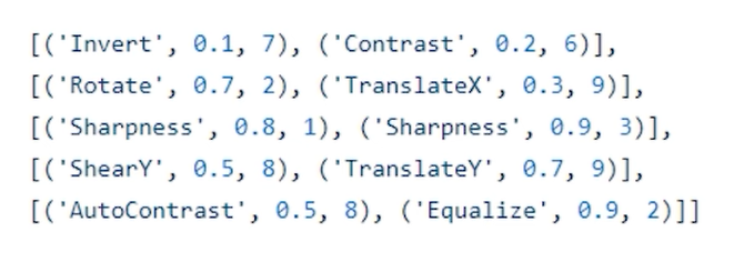
data로 부터 data augmentation 전략을 학습하는 또 다른 접근방식은 AutoAugment로 강화학습 을 이용하여 sequence of operation과 적용 확률 및 규모를 선택함. 위 그림은 sub-policy가 적용될 확률 및 크기

  • AutoAugment policy 적용에는 여러가지 확률 적용. 다음과 같은 절차를 거쳐서 적용한다.
    1. 모든 minibatch의 모든 이미지에 대해 uniform probability로 sub-policy가 선택.
    2. 각 sub-policy에서의 동작에는 확률이 있음.
    3. 일부 연산은 방향에 대한 확률을 가진다.
      • 예를 들면 이미지를 시계방향이나 시계반대 방향으로 회전
  • 확률을 이용하여 network훈련되는 다양성을 증가 시키고, 이는 많은 데이터셋에서 generalization을 크게 개선

PBAFast Autoaugmentautoaugment에서 더 좋은 방법을 찾기 위해 노력한 결과물이다.

  • 시간은 줄어들었지만 별도의 search phase가 있어서 문제.
  • 이 논문에서는 별도의 proxy task에서 search phase를 제거하는 것을 목표로함

3. Methods

RandAugment의 목표는 proxy task에서 별도의 search phase가 필요하지 않도록 하는것.

  • proxy task란 본래의 목적을 달성하기 위한 부가적인 task를 말함.
  • Search phase를 없앨려는 이유는 별도의 search phase가 training을 복잡하게됨.
  • 그리고 계산량이 많아지는 안좋은 현상이 존재.
  • 그리고 proxy task가 꼭 최선의 결과를 얻는것도 아님!!.

이전에 augmentation 방법들은 30개 이상의 하이퍼파라미터를 포함 해야했음.

  • 저자들은 parameter space을 크게 줄이는데 초점을 맞춤.

                                                          변환 적용 확률을 열거한 것.
  •  
  • 이전 연구에서는 다음과 같이 변환중에 변환을 선택하고 각 변환을 적용할 확률을 열거함.

그러면 RandAugment에서는 어떤 parameter만을 사용하느냐?

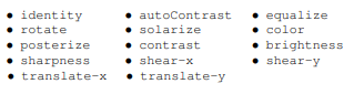
  1. 첫번째 parameter로는 augmentation을 적용할 변환의 개수(N), 논문에서는 14개 선택.
  • parameter space를 줄이면서 이미지의 다양성을 유지하기 위해 각 변환을 적용하는 확률은 균일한 확률인 1/K.

       저자들이 적용한 변환의 종류 총 14개
  • Training image에 N개이 변환이 주어지면 RandAugment의 경우에는 K^N개의 정책을 선택할 수 있음.
  1. 그리고 마지막 Parameter는 distortion(왜곡)의 크기(M)
  • 왜곡의 크기란 그림으로 이해하는게 더 쉬움

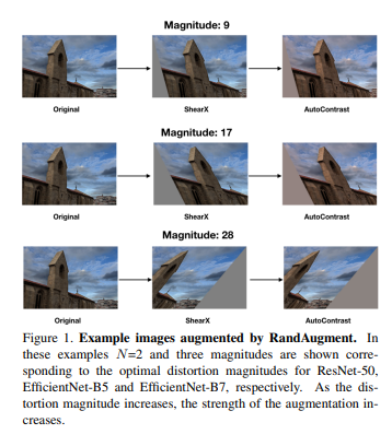
                Figure1. Example RandAugment
  • 위 의 그림은 보면 N = 2 이고, M은 한줄씩 9,17,28를 적용한 예 값이 커질수록 그림의 왜곡이 심해지는 것을 알 수 있다. 논문에서는 0~10 사이로 M을 정한다고 합니다.
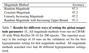
  • 저자들은 M을 선택하는 방식을 여러개로 구분하여 Test Random, Constant, Linear Increasing, Random Magnitude로 Test 성능이 0.1% 정도 거의 차이가 나지 않는 다는 것을 알 수 있다.

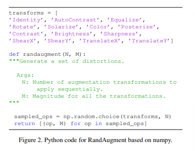
  1. 알고리즘은 다음과 같이 아주 간단한 파이썬 코드로 구현가능하다.

                       Python Based Numpy 구현
  • 코드가 매우 간단하며 인간이 해석하기 편하고 N,M이 커질수록 regularization strength이 커짐 ( Data가 더욱더 다양해 지므로)
  • N,M을 선택하기 위해 다른방법도 선택 할 수 있지만 저자들이 개발한 것은 매우 작은 search space를 고려할 때 naive grid search가 효과적이라고 함. Grid search (격자 탐색) 은 모델 하이퍼 파라미터에 넣을 수 있는 값들을 순차적으로 입력한뒤에 가장 높은 성능을 보이는 하이퍼 파라미터들을 찾는 탐색 방법이다.

4. Results

본 논문에서는 small proxy task에서 data augmentation policy를 찾는것이 문제라고함 모델 사이즈와 data set 사이즈가 두가지 측면에서 이를 분석함

  • 그림을 보면 왼쪽위를 보면 distortion magnitude에 따른 성능을 확인 할 수 있음.
    • 사각형이 표시 된 것이 최적의 Magnitude인것을 암시함.
    • network size가 클수록 큰 distortion Magnitude에서 좋은 성능을 보임.
    • 위의 결과로 알 수 있는 것은 small proxy task에서 distortion Magnitude 찾는것은 부적절함
  • 왼쪽 밑에 그림은 widening, 네트워크 사이즈에 따른 결과임.
    • Parameter가 커질 수록 distortion 이 커져야 성능이 좋아지는 것을 알 수 있음.
  • 오른쪽은 training data set 사이즈 에 대한 결과임.
    • 확인하면 **1k인 파란색에서는 3%**정도. 4k인 것은 2%, **10k인 것은 약 1.5%**만 성능이 좋아짐.
  • 오른쪽 아래를 보면 data set의 사이즈가 클수록 optimal distortion magnitude가 커짐.
    • 이는 작은 data set에서 더 큰 Regularization이 필요할거 같다는 예상과는 일치안함
    • 이 결과는 중요한 점이 있음. 더 큰 data set에서는 더 강한 augmentation이 필요함. 일부만으로 파악하는 proxy task에는 문제가 있음. proxy task에서 한 policy는 전체 training data에는 적용하기 안좋은 것을 알 수 있음.
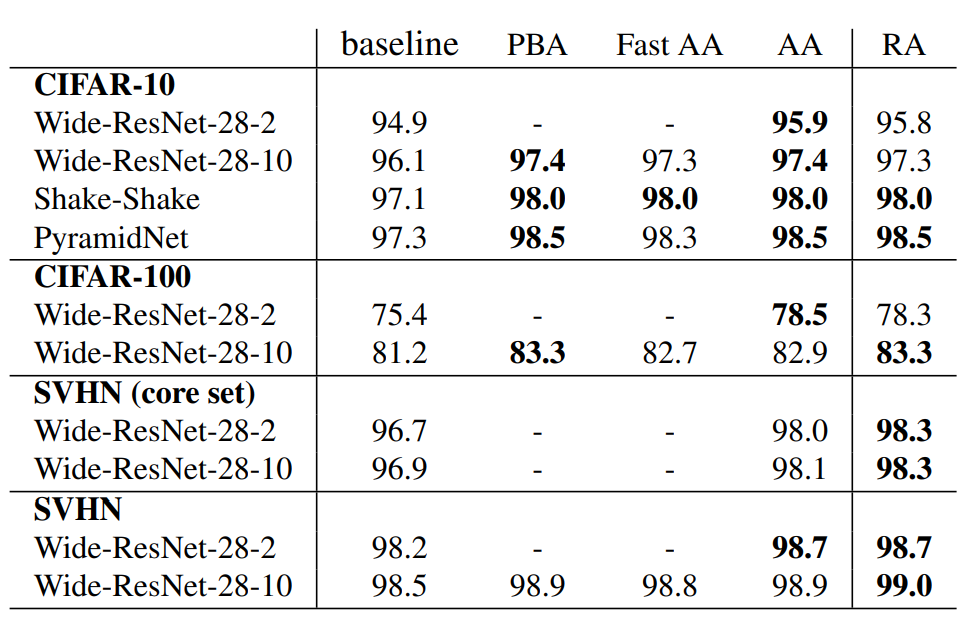
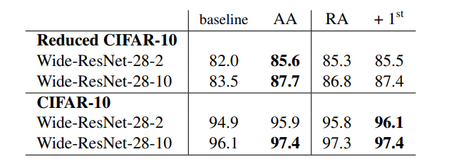
CIFAR와 SVHN에서 결과

  • CIFAR , SVHN에서 결과는 다음과 같다.
  • RA는 PBA, FAST AA, AA에 비해 성능이 꿀리지 않고, 몇몇은 제일 좋은 것을 알 수 있음.
  • CIFAR와 SVHN은 아예다른 이미지를 가지고 있음. Fast AA나 ,AA에서의 Policy는 많이 다른 결과가 나왔다고 한다.
    • 즉 data augmentation policy 가 많이 달라도 RandAugment는 동일 또는 더 좋은 성능이 나오게 된다는 것을 알 수 있음.
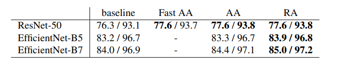
IMAGENET에서 결과

  • 모델에서 성능을 개선하는 data augmentation이 항상 imagenet과 같은 데이터셋에서 성능을 좋게 하는 것은 아님.
  • 항상 성능을 향상시키는게 아니거나 거의 변화가 없었다.

COCO에서 결과

  • object detection은 다음과 같은 결과가 나온 것을 알 수 있다.
  • Auto augment에서는 randAugment에서 사용하지 않은 변환도 사용하도록 하였다.
  • 그리고 굉장히 큰 Search space, GPU연산량이 들어도 6개의 value의 하이퍼 파라미터 튜닝한 RandAugment와 비슷한 결과가 나온 것을 알 수 있다.
  • 이 실험에서는 RandAugment가 bbox에서도 적용가능한 transformation이 제한되어 있어 더 다양한 변환이 필요하다고 함.
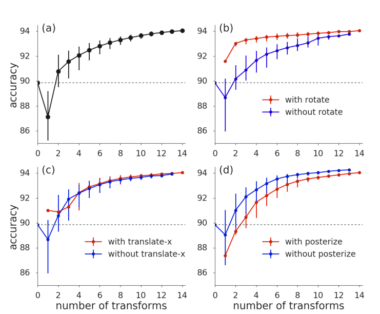
변환 개수에 따른 결과

모든 결과는 CIFAR-10 기준이다.

  • (A)
    • 그래프 A를 보면 변환이 많으면 성능이 높아짐.
  • (B)
    • 그래프 B를 보면 rotate가 성능에 큰 영향을 미친 다는 것을 알 수 있음.
  • (C)
    • 그래프 C를 보면 translate는 생각보다 큰 영향을 미치지 않는 것을 알 수 있음.
  • (D)
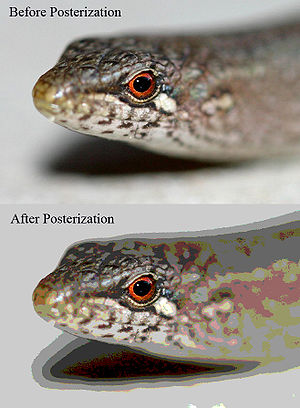
    • 그래프 D를 보면 poseterize는 성능이 안좋아지는 것을 알 수 있음. (이미지 음영을 조절하는것,아래 그림은 poseterize의 결과)
     

다른 결과

  • 위의 결과는 확률을 학습하면 성능이 좋아진다고 생각했으며, 작은 data set에서 테스트를 한 것.성능이 향상된것을 확인할 수 있었으며, 큰 data set에 대해선 차후 과제로 남겨두었습니다.

5. Discussion

  • data augmentation은 최고의 성능을 위해 필수
  • 학습된 data augmentation 전략을 자동화 하여 성능을 높임
  • 별도의 search 없이 기존연구와 비슷하거나 좋은 성능을 얻음
  • 기존의 연구는 큰 data set에서는 적용이 힘들지만 두개의 hyperparameter를 이용하여 좋은 성능을 얻음


Using RandAugment

Unofficial Pytorch Reimplementation of RandAugment 카카오 브레인 김일두

GitHub - ildoonet/pytorch-randaugment: Unofficial PyTorch Reimplementation of RandAugment.


GitHub - ildoonet/pytorch-randaugment: Unofficial PyTorch Reimplementation of RandAugment.

Unofficial PyTorch Reimplementation of RandAugment. - GitHub - ildoonet/pytorch-randaugment: Unofficial PyTorch Reimplementation of RandAugment.

github.com

RandAugment가 구현된 부분은 다음과 같다.

pytorch-randaugment/augmentations.py at master · ildoonet/pytorch-randaugment


GitHub - ildoonet/pytorch-randaugment: Unofficial PyTorch Reimplementation of RandAugment.

Unofficial PyTorch Reimplementation of RandAugment. - GitHub - ildoonet/pytorch-randaugment: Unofficial PyTorch Reimplementation of RandAugment.

github.com

Python Imaging Library를 이용하여 구현

pip install git+https://github.com/ildoonet/pytorch-randaugment

명령어를 입력하여 설치 가능.

from torchvision.transforms import transforms
from RandAugment import RandAugment

transform_train = transforms.Compose([
    transforms.RandomCrop(32, padding=4),
    transforms.RandomHorizontalFlip(),
    transforms.ToTensor(),
    transforms.Normalize(_CIFAR_MEAN, _CIFAR_STD),
])

# Add RandAugment with N, M(hyperparameter)
transform_train.transforms.insert(0, RandAugment(N, M))

다음과 같이 transform에 N,M Hyperparameter를 조절하여 insert한다.

Google Colaboratory


RandAugment.ipynb

Colaboratory notebook

colab.research.google.com


https://inha-kim.tistory.com/47


[논문 리뷰] ResNet (2015) 논문리뷰 (Deep Residual Learning for Image Recognition)

https://arxiv.org/pdf/1512.03385.pdf 논문 링크 입니다. 이제 4개째 CNN논문 리뷰네요. 다음에는 좀 다른 유형의 논문을 리뷰 할 계획입니다. 감사합니다 _-_ 2015년에 압도적인 성능개선으로 ILSVRC를 우승 한

inha-kim.tistory.com

이 그림을 참고하여 구현 하였습니다.
https://github.com/weiaicunzai/pytorch-cifar100/blob/master/models/resnet.py


GitHub - weiaicunzai/pytorch-cifar100: Practice on cifar100(ResNet, DenseNet, VGG, GoogleNet, InceptionV3, InceptionV4, Inceptio

Practice on cifar100(ResNet, DenseNet, VGG, GoogleNet, InceptionV3, InceptionV4, Inception-ResNetv2, Xception, Resnet In Resnet, ResNext,ShuffleNet, ShuffleNetv2, MobileNet, MobileNetv2, SqueezeNet...

github.com

이 코드 구현을 참고

1
2
3
4
5
6
7
8
9
10
11
12
13
14
15
16
17
18
19
20
21
22
23
24
25
26
27
28
29
30
31
32
33
34
35
36
37
38
39
40
41
42
43
44
45
46
47
48
49
50
51
52
53
54
55
56
57
58
59
60
61
62
63
64
65
66
67
68
69
70
71
72
73
74
75
76
77
78
79
80
81
82
83
84
85
86
87
88
89
90
91
92
93
94
95
96
97
98
99
100
101
102
103
104
105
106
107
108
109
110
111
112
113
114
115
116
117
118
119
120
121
122
123
124
125
126
127
128
129
130
131
132
133
134
import torch
import torch.nn as nn
from torchsummary import summary
 
class BasicBlock(nn.Module):
    # ResNet Basic Block으로 18, 34 layer에 들어가는 것들이다.
    # dimension 이 달라지는 경우
    dimension_expansion = 1  
    # size 축소시에 stride=2로 전달받음
    def __init__(self,in_channels,out_channels,stride=1):
        super().__init__()
        # stride = 1인 경우 size 유지, stride가 2 인 경우 size 2로 나눠짐
        self.residual_function = nn.Sequential(
            nn.Conv2d(in_channels, out_channels, kernel_size=3,stride=stride,padding=1,bias=False),
            nn.BatchNorm2d(out_channels),
            nn.ReLU(inplace=True),
            nn.Conv2d(out_channels, out_channels * BasicBlock.dimension_expansion, kernel_size=3,stride=1,padding=1,bias=False),
            nn.BatchNorm2d(out_channels * BasicBlock.dimension_expansion),
        )
        # Shortcut 
        self.shortcut = nn.Sequential()
        if stride != 1 or in_channels != out_channels * BasicBlock.dimension_expansion:
            self.shortcut = nn.Sequential(
                nn.Conv2d(in_channels, out_channels * BasicBlock.dimension_expansion, kernel_size = 1,stride = stride, bias=False),
                nn.BatchNorm2d(out_channels * BasicBlock.dimension_expansion),
            )
        # input, output 결합
        self.relu = nn.ReLU(inplace=True)
    
    def forward(self,x):
        out = self.residual_function(x) + self.shortcut(x)
        out = self.relu(out)
        return out
 
class BottleNeck(nn.Module):
  ㄱ # ResNet BottleNeck Block으로 50,101,152 layer에 들어가는 것들이다.
    # dimension 이 달라지는 경우가 존재, 4배로 커지는 경향이 있음
    dimension_expansion = 4
    # size 축소시에 stride=2로 전달받음
    def __init__(self,in_channels,out_channels,stride=1):
        super().__init__()
        self.residual_function = nn.Sequential(
            nn.Conv2d(in_channels,out_channels,kernel_size=1,stride=1,bias=False),
            nn.BatchNorm2d(out_channels),
            nn.ReLU(inplace=True),
            nn.Conv2d(out_channels,out_channels,kernel_size=3,stride=stride,padding=1,bias=False),
            nn.BatchNorm2d(out_channels),
            nn.ReLU(inplace=True),
            nn.Conv2d(out_channels,out_channels*BottleNeck.dimension_expansion,kernel_size=1,stride=1,bias=False),
            nn.BatchNorm2d(out_channels*BottleNeck.dimension_expansion),
        )
        self.shortcut = nn.Sequential()
        if stride != 1 or in_channels != out_channels * BottleNeck.dimension_expansion:
            self.shortcut = nn.Sequential(
                nn.Conv2d(in_channels, out_channels * BottleNeck.dimension_expansion, kernel_size = 1,stride = stride, bias=False),
                nn.BatchNorm2d(out_channels * BottleNeck.dimension_expansion),
            ) 
        self.relu = nn.ReLU(inplace=True)
    
    def forward(self,x):
        out = self.residual_function(x) + self.shortcut(x)
        out = self.relu(out)
        return out
 
class ResNet(nn.Module):
    # ResNet class
    def __init__(self,block_type,num_blocks,num_classes=10):
        super().__init__()
        self.in_channels = 64
        
        self.conv1 = nn.Sequential(
            nn.Conv2d(3,64,kernel_size = 7,stride = 2,padding = 3,bias=False),
            nn.BatchNorm2d(64),
            nn.ReLU(inplace=True),
            nn.MaxPool2d(kernel_size=3,stride=2,padding=1)       
        )
        # maxpool2d가 사실 conv2_x에 속해서 size를 반으로 줄임,그러므로 stride=1로 전달
        self.conv2_x = self.make_layer(block_type,64,num_blocks[0],1)
        self.conv3_x = self.make_layer(block_type,128,num_blocks[1],2)
        self.conv4_x = self.make_layer(block_type,256,num_blocks[2],2)
        self.conv5_x = self.make_layer(block_type,512,num_blocks[3],2)
        self.avg_pool = nn.AdaptiveAvgPool2d((1,1))
        self.fc = nn.Linear(512 * block_type.dimension_expansion ,num_classes)
 
    def make_layer(self,block_type,out_channels,num_block,stride):
        # stride가 2 일 경우 list 맨 앞만 2, 나머진 1
        strides = [stride] + [1* (num_block-1)
        layers = []
        for stride in strides:
            layers.append(block_type(self.in_channels,out_channels,stride))
            self.in_channels = out_channels * block_type.dimension_expansion
        return nn.Sequential(*layers)
    
    def forward(self,x):
        out = self.conv1(x)
        out = self.conv2_x(out)
        out = self.conv3_x(out)
        out = self.conv4_x(out)
        out = self.conv5_x(out)
        out = self.avg_pool(out)
        out = out.view(out.size(0),-1)
        out = self.fc(out)
        return out
 
def resnet18():
    """ return a ResNet 18 object
    """
    return ResNet(BasicBlock, [2222])
 
def resnet34():
    """ return a ResNet 34 object
    """
    return ResNet(BasicBlock, [3463])
 
def resnet50():
    """ return a ResNet 50 object
    """
    return ResNet(BottleNeck, [3463])
 
def resnet101():
    """ return a ResNet 101 object
    """
    return ResNet(BottleNeck, [34233])
 
def resnet152():
    """ return a ResNet 152 object
    """
    return ResNet(BottleNeck, [38363])
 
 
device = torch.device('cuda' if torch.cuda.is_available() else 'cpu')
print(device)
model = resnet50().to(device)
summary(model, (3224224), device=device.type)
cs

+ Recent posts